Molecular dynamics can tell you a lot about a material — diffusivity, structural correlations, thermal properties — but every one of those measurements assumes you started from a well-equilibrated structure. For polymers, getting to that starting point is surprisingly hard. This post walks through two practical protocols for equilibrating a polymer melt, both adapted from published work and both runnable end-to-end in Jungular.
If you'd rather follow along with the exact files, grab them here:
Why polymers are hard to pack
For a simple liquid like water, generating an initial configuration is easy: scatter molecules into the box by sampling positions from a uniform distribution and reject any that overlap. When two molecules land too close, the energy blows up — so you just try again. With enough empty space, this "click, click, click" placement works fine.
Polymers break this approach. A single chain of even ~40 carbons is already awkward to place, and once you have a handful of chains in the box, squeezing in another one becomes nearly impossible without expensive tricks — rotating parts of the chain, Monte Carlo moves, and so on. Chains get in each other's way in a way that small molecules never do.
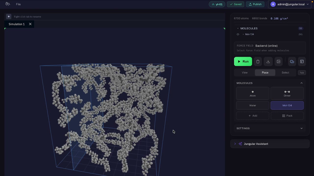
The standard workaround is to start from a low-density box. Pack your chains into a box that's much larger than the target — say 50 chains in a 50 Å box — so there's plenty of room and no overlaps. The catch: that configuration is nowhere near the density of a real polymer at room temperature and pressure. So the real work is driving the system from that sparse starting point down to the correct target state. Both methods below do exactly that, using a series of short MD simulations.
Method 1: Slow compression
The first protocol is adapted from a study of PIM-1, a polymer of intrinsic microporosity. The paper lays out a detailed recipe for taking a low-density initial structure and compressing it to a representative equilibrated state. The logic is worth understanding, not just copying.
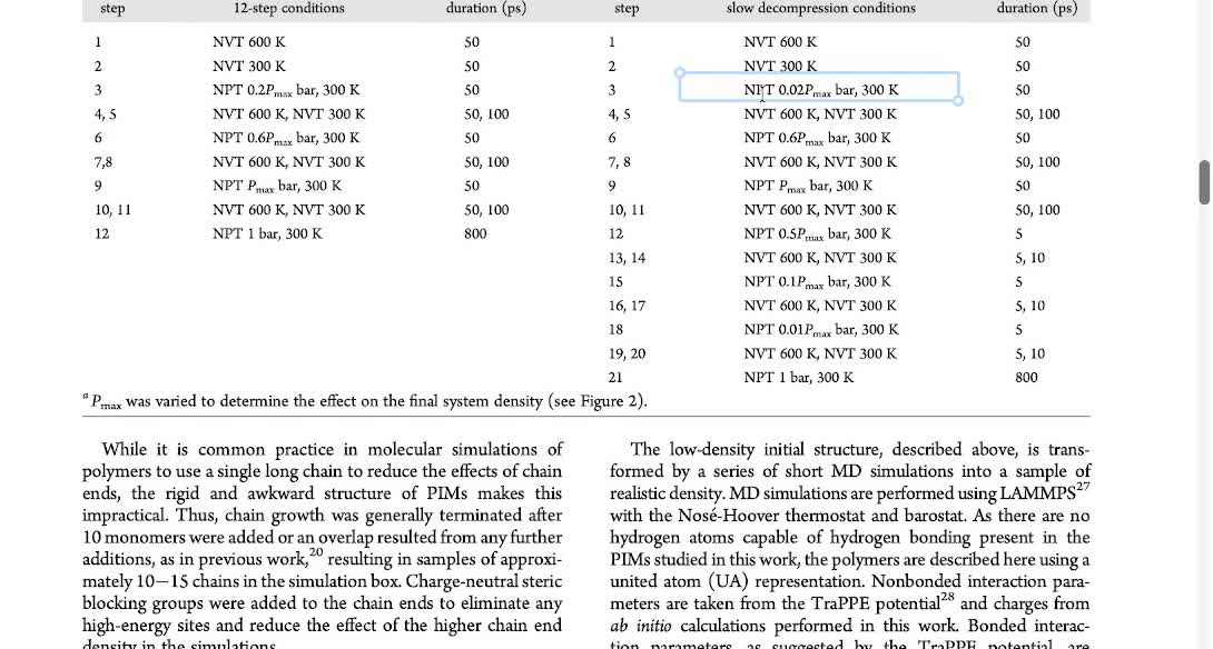
Start hot, in a fixed box. The first steps run under NVT (fixed volume, fixed temperature) at 600 K — well above the glass transition of most polymers. Why so hot? If your initial structure is poor, the system can get trapped in a local energy minimum. At 300 K it may never escape; the extra thermal energy at 600 K lets the atoms move around freely and relax the structure. After the hot NVT step, the system is cooled to 300 K and relaxed further. Because the volume is fixed in these steps, the density hasn't changed yet — this is purely about untangling the structure.
Then squeeze, gradually. Now the protocol switches to NPT, where pressure is fixed and the box volume is free to change. To collapse the empty space, it applies pressure in stages: 2% of P_max, then 60%, then 100%, where P_max is a very high 50,000 bar (for reference, atmospheric pressure is about 1 bar). Between compression steps, short NVT runs relax the structure before the next squeeze.
Why ramp the pressure up instead of slamming the box with 50,000 bar from the start? Stability. Early on, the structure isn't robust; jumping straight to maximum pressure makes atoms move violently, and once two atoms get too close the forces spike, atoms fly apart, and the simulation dies. Gradual compression keeps things under control.
Then decompress to the real target. After reaching P_max and squeezing out essentially all the empty space, the pressure is walked back down to 1 bar — the actual state we care about — with a long final NPT run (800 ps, much longer than the earlier steps, because this is the state we want to sample).
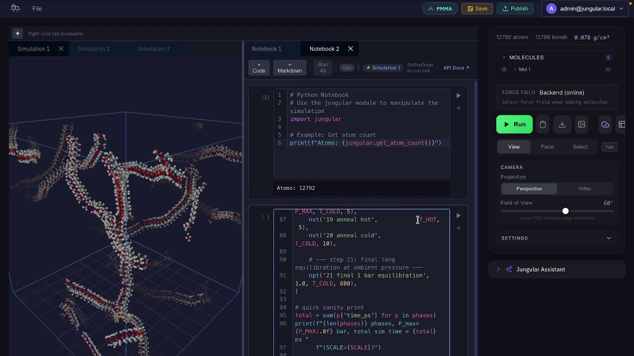
In Jungular, the whole thing is expressed as a list of NVT and NPT phases — 21 steps in total — built with simple helper functions that each return the ensemble, temperature, pressure, and duration. The phase UI lays out every step so you can sanity-check the protocol, and the generated LAMMPS script is right there to review before you submit to the cloud.
Method 2: Slow cooling
The second protocol is inspired by a high-throughput study that computed glass transition temperatures for 315 polymers. Their Tg method cools the system from a high temperature in small steps while tracking density — and even though we don't care about Tg here, the cooling idea is exactly what we need.
The recipe is simpler than Method 1: equilibrate, then cool. After an initial NPT stage to squeeze out the worst of the empty space and relax the structure, you cool the system down from a high starting temperature in fixed increments, running NPT at each step. The original paper cooled from 1000 K to 100 K in 20 K steps at 5 ns each; here we start at 600 K (we only need the equilibrium structure at 300 K, not the full Tg curve) and cool in steps toward room temperature, running 3 ns per step to keep the compute cost manageable.
In the notebook this is just an array of temperatures, reversed into decreasing order, looped over to build the NPT phases. The phase UI shows the initial equilibration stage followed by each cooling step, and again the generated LAMMPS script is there to inspect before submitting.

What the results actually look like
To test both methods, the video uses PMMA — long chains totaling about 12,000 atoms — with three independent starting configurations so we can put an error bar on the answer.
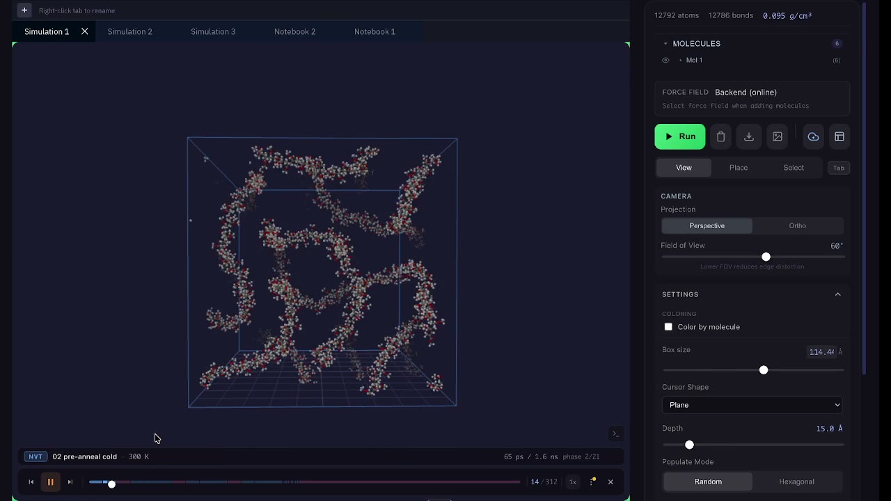
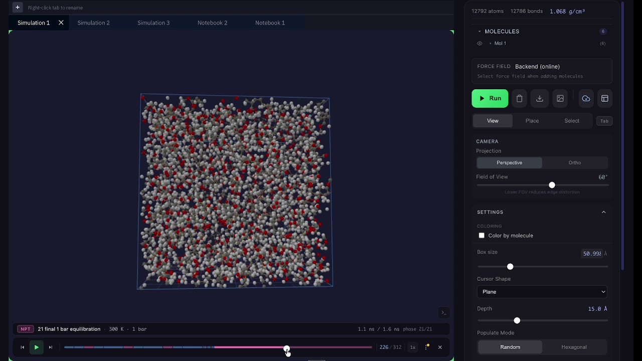
Method 1 shows exactly the expected behavior on playback: density stays low (~0.29 g/cm³) through the initial fixed-volume stages, then climbs sharply as compression begins, reaching ~1.4 g/cm³ at P_max (50,000 bar), before settling around 1.03–1.06 g/cm³ once decompressed to 1 bar. Two samples run under the identical protocol landed at 1.03 and 1.06 — a reminder that the initial configuration matters, and why reporting an error bar isn't optional.
Method 2 cools over a much longer trajectory (~54 ns vs. ~1.6 ns for Method 1) and gives densities around 1.06–1.07 g/cm³ at 300 K — in the same ballpark as Method 1, though with only two samples per method it's hard to say which is systematically higher.
A note on accuracy: the experimental density of PMMA is around 1.18 g/cm³, and these simulations come in below that. Two likely reasons — the force field (OpenFF here, not trained specifically on polymers) and limited sampling. These runs are expensive; a single simulation can take days. The point of the video isn't a perfectly converged number, it's the process: a repeatable way to take a sparse initial box to an equilibrated polymer melt.
A word on error bars
Because two runs of the same protocol gave different densities, running just one simulation would give you a number you can't trust. Multiple independent samples let you estimate the uncertainty — and if you want a tighter error bar, run more samples (doubling the number of runs shrinks the error by roughly √2). Whenever you see a reported value with no error bar, be skeptical.
Try it yourself
Both protocols — the full LAMMPS control scripts for slow compression and slow cooling, plus the polymer structure files — are available to download:
If you run into issues or have questions, reply to the email you'll get with the files — I read and answer every one. And if you'd like more molecular simulation walkthroughs, subscribe to stay in the loop.